
Technical Note
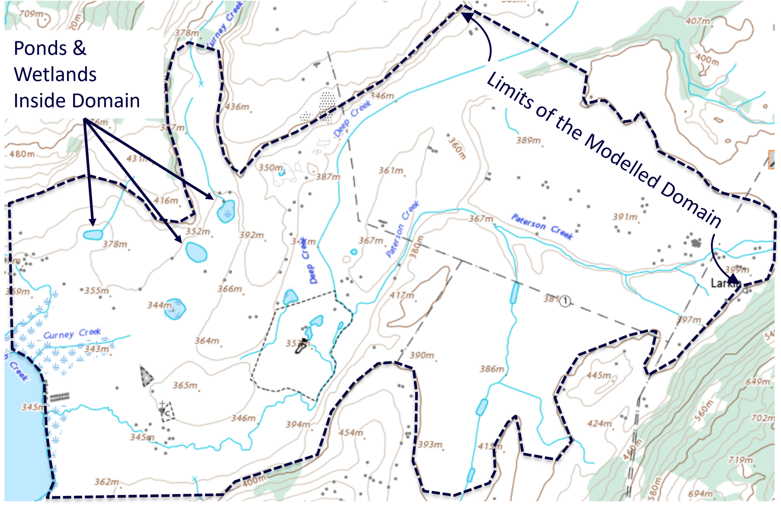
Lakes, ponds, and wetlands are common features in groundwater problems. In many projects, you need to represent them inside the model domain. In Anaqsim, you can represent these non-linear surface water features in three main ways: the Subdomain Method, the Line Boundary Method, and the Surface Polygon Method.
This article is a practical guide to those three methods. It explains what each method does, where each one tends to work well, and how to choose a sensible starting point for your model.
What Anaqsim is simulating and what it is not
First we need to be clear that Anaqsim simulates groundwater, not full surface-water hydraulics.
However, in most groundwater projects, you do not need to simulate every detail of circulation inside a pond, lake, or wetland. The more practical question is usually how that feature interacts with the aquifer. Does it recharge groundwater? Does it receive groundwater discharge? Could pumping cause it to leak more strongly, or even dry up?
With the right setup, Anaqsim can represent the hydraulic effects of lakes, ponds, and wetlands inside the model domain. That is often enough for engineering and hydrogeologic work.

Subdomain Method
The Subdomain Method is the most flexible of the three. In this method, you represent an overlying lake, pond, or wetland by applying either a specified flux or a head-dependent flux to the top of a subdomain using recharge nodes. The subdomain boundary defines the shape of the surface water feature.
A subdomain acts as its own model zone. That means you can vary thickness, add layers, and assign different aquifer properties as needed. This method is especially useful when vertical flow between the surface water and the aquifer is important to the assessment. There are two general approaches to the subdomain method.
If subdomains are new to you, Basic Tutorial 2 is a good companion to this section. It walks through adding new domains and using an interdomain boundary to define a multi-layer region.
1. Surface effect on top of the subdomain
In the first approach, the subdomain defines the shape of the lake, pond, or wetland. It still represents the aquifer beneath the surface water. You then apply the surface water effect to the top of that subdomain using recharge nodes. This can be done with either a specified flux or a head-dependent flux.
This is often a good choice for shallow surface water features. Use it when you want to apply the hydraulic effect at the model surface, not simulate the water body itself in detail. You can also split the subdomain into multiple layers if needed, so the model can include 3D vertical flow.
Model Input → Area Source/Sink → Uniform, Domain
For steady, single-layer models, a specified flux can be entered through:
For multi-layer or transient setups, use:
Model Input → Area Source/Sink → Spatially-Variable, Domain
2. Subdomain as the water body
In the second approach, the geometric setup is similar. But here, the subdomain itself represents the surface water body instead of the aquifer beneath it. In effect, you “fill” the subdomain with surface water by assigning material properties that behave more like free-flowing water than aquifer material.
This lets the model respond to head changes within the water body itself rather than only applying a surface effect at the top of the model. It is often the better choice when you want to simulate behavior around the surface water body, such as pit-lake rebound in a quarry or mine or the impacts of dewatering.
You will find the key inputs for this approach under Model Input → Domains, just like any other domain in the model.
If the subdomain representing the water body has only one layer, its full thickness represents the surface water body. That is equivalent to a fully penetrating lake or pond. If the feature should only partially penetrate, split the subdomain into two or more layers. Then let the upper layer represent the surface water and the lower layer or layers represent the aquifer below.
When the Subdomain Method is often the best choice
This method can be used in single-layer models. However, it is often the best choice in multi-layer models where the water body can be simulated and/or 3D vertical flow can be included in the model. It also gives you the most detailed representation of the surface water body. For that reason, it is usually the best choice when groundwater interaction with the feature is central to the purpose of the model.
Line Boundary Method
The Line Boundary Method uses a closed line boundary to represent the surface water feature. That line acts like a fence around the lake, pond, or wetland. You place that fence within the aquifer layer, and it fully penetrates that layer. Instead of creating a separate subdomain, you define the shape with a line and let that line control how the feature interacts with the aquifer.
This method is simpler than the subdomain method because you do not need to create a separate internal zone. The tradeoff is that the line enforces the surface water effect directly within the layer. That makes the response more fixed than in the subdomain approach. It also creates a fixed shape for the surface water body, which can be useful when that kind of strong geometric control is desired in the model. There are two main approaches within the line boundary method.
1. Head-Specified Line Boundary
A Head-Specified Line Boundary fixes the water level along the boundary. Anaqsim then computes whatever discharge is needed to maintain that specified head.
For internal surface water features, this is the simplest line-based option when you mainly want to hold the feature at a known stage.
The setup path is:
Model Input → Line Boundaries → Head-Specified
2. River Line Boundary
A River Line Boundary is similar, but it adds one important feature: Dries_up. With Dries_up checked, discharge per unit length becomes zero when the aquifer head drops below stage. The boundary then stops supplying water to the aquifer. This makes it useful for small surface water features that could dry up under stresses such as pumping.
The river boundary also uses stage, conductance, and the base of the resisting layer as its core inputs. These inputs were designed for streams and rivers, but the default setup usually works well for lakes, ponds, and wetlands too.
The setup path is:
Model Input → Line Boundaries → River
When the Line Boundary Method is often a good fit
This method is often a good fit for single-layer or regional-scale models where detailed 3D effects around the surface water body are not of interest. It is also a sensible starting point when a simpler line-based approximation is sufficient. The Head-Specified Line Boundary is usually the more direct fixed-stage option. The River Line Boundary is usually the better choice when dry-up behavior needs to be tested.
Surface Polygon Method
The Surface Polygon Method draws the surface water footprint as a polygon on top of an existing domain. It then applies either a specified flux or a head-dependent flux over that area with recharge nodes. No separate subdomain or line boundary is required.
This is the simplest of the three methods to add and remove because the effect is applied only at the model surface. That makes it a practical option when you want to test ideas quickly.
The setup path is:
Model Input → Area Source/Sink → Spatially-Variable, Polygon
From there, you can apply the polygon either a specified flux or a head-dependent flux over the selected area.
When the Surface Polygon Method is often a good fit
This method is often a good fit when you want a quick surface-only approximation of the hydraulic effect of a lake, pond, or wetland. It can be especially useful when the feature straddles two or more existing geological zones, because no new internal boundaries are needed to match its shape.
It is the quickest and simplest of the three methods, but it is also the most approximate. In many cases, that is perfectly acceptable, especially when you are testing ideas, screening alternatives, or only need the general surface water effect.
A practical way to choose
A good starting point is to ask a simple question: How much do I need this surface water feature to behave like a real part of the groundwater system?
The more detailed and responsive that behavior needs to be, the more likely the Subdomain Method is the right starting point. The more approximate the effect can be, the more likely a Line Boundary or Surface Polygon approach will be enough.
Just as important, you do not need to worry too much about choosing the “perfect” method at the start. One of Anaqsim’s practical strengths is that these kinds of features can be revised with relatively little effort. A surface polygon can be replaced with a line boundary, or a line boundary can be developed into a subdomain, if the model later needs a more detailed representation.
A practical rule of thumb is this: start with the simplest method that is still credible for the question you are trying to answer. If that first setup does not capture enough of the behavior you care about, then move to the next level of detail.
Final thoughts
Anaqsim gives you several practical ways to represent lakes, ponds, and wetlands inside the model domain. The best choice depends on what role the surface water feature plays in the problem and how much detail the model needs to answer that problem well.
A sensible workflow is to begin with the simplest method that still fits the purpose of the model. Then add detail only if the problem calls for it. it.
Further Reading
Fitts, C. R. (2010). Modeling aquifer systems with analytic elements and subdomains. Water Resources Research, 46, W07521. DOI: 10.1029/2009WR008331
Strack, O. D. L., & Janković, I. (1999). A multi-quadric area-sink for analytic element modeling of groundwater flow. Journal of Hydrology, 226(3-4), 188–196. DOI: 10.1016/S0022-1694(99)00147-4
Fitts, C. R. (2023). Groundwater Science (3rd ed.). Academic Press. Print ISBN: 978-0-12-811455-1. eText ISBN: 978-0-12-811456-8. Book page: Groundwater Science, 3rd Edition