
Every groundwater model depends on a conceptual model.
Before you build the model, you first decide what controls groundwater flow. A river crosses the site, a wellfield pumps from the aquifer, recharge enters from above, and a drain lowers groundwater near a slope. In another project, the important controls may be a pit, tunnel, lake, boundary, or low-permeability zone.
At this stage, you usually describe the groundwater system in familiar hydrogeologic terms. You have not yet translated the model into software, but the main flow controls are already visible.
That translation step is where modelling methods begin to differ.
A finite difference model translates the conceptual model into grid cells. A finite element model translates it into a mesh. The analytic element method, or AEM, translates it into groundwater features.
That is the central idea behind AEM:
The analytic element method turns the hydraulic and geological features in the conceptual model into the structure of the groundwater model.
How AEM represents groundwater features
AEM represents the features that control groundwater flow as model elements.
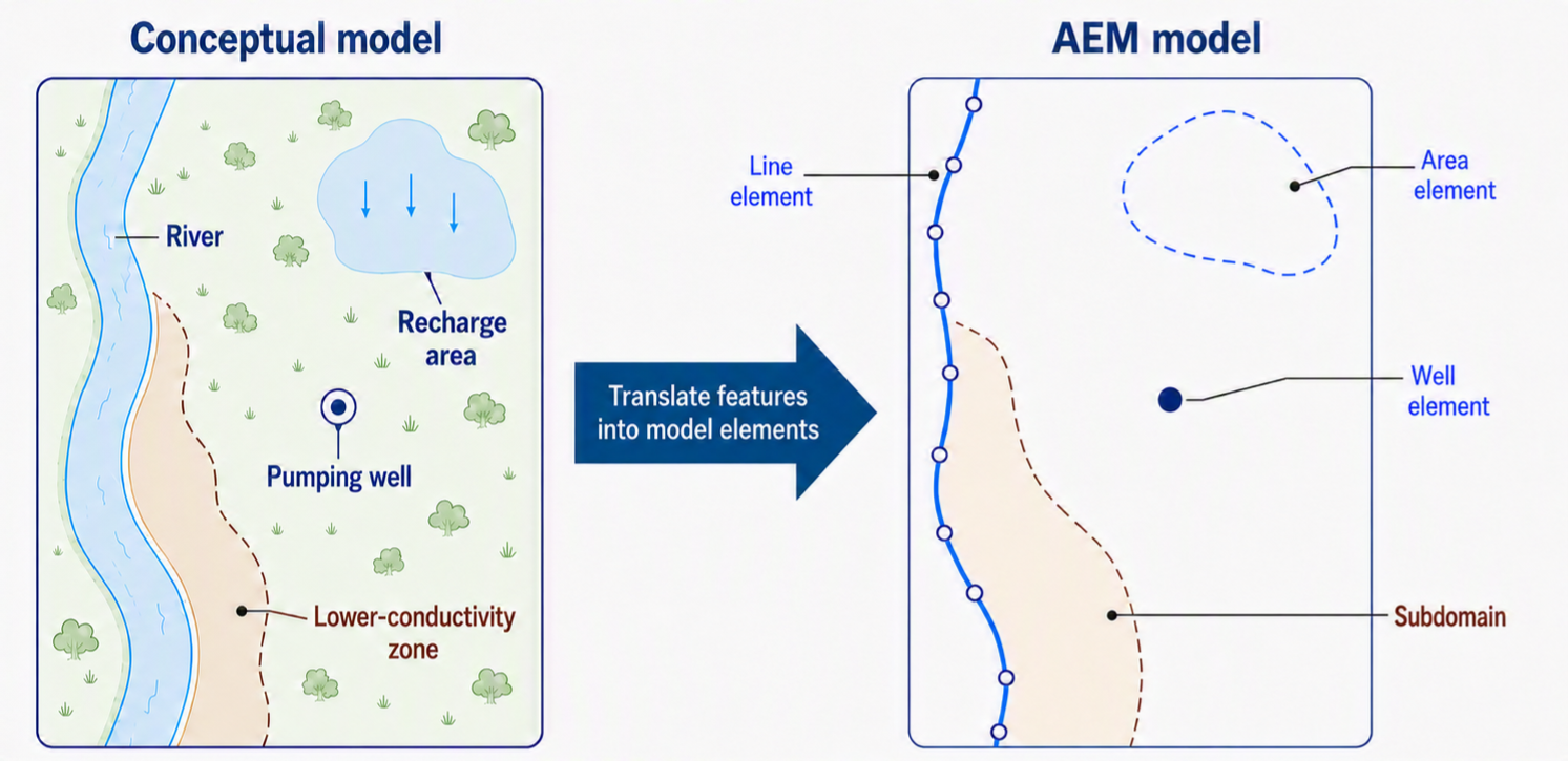
For example, a pumping well becomes a well element, while a river becomes a line element. Recharge areas become area elements, drains become drainage elements, and low-permeability barriers become barrier elements. You can also represent zones with different hydraulic conductivity, aquifer thickness, storage, anisotropy, or base elevation as distinct aquifer zones or subdomains.
The model is still mathematical, and the inputs still require judgement. Even so, the translation from conceptual model to model structure can be unusually direct because you can begin with a familiar question:
What features control groundwater flow?
That question is often close to the way the conceptual model was built in the first place.
How the elements combine
Each AEM element contributes to the groundwater solution in a specific way.
A pumping well lowers the groundwater surface around it, while an injection well raises it. Rivers can add or remove water depending on the nearby groundwater head. Recharge areas add water across an area, drains remove water when groundwater rises above the drain level, and subdomains change the flow field where aquifer properties change.
AEM combines these effects using superposition.
Superposition means the total solution is built by adding individual contributions together. This idea is familiar from many classic groundwater equations and is widely used in physics wherever individual effects can be added together. AEM extends the same principle by combining many analytic elements in one model.
As a result, AEM can sit between hand calculations and large numerical models. A closed-form equation may give a clean answer for one idealized condition, while AEM keeps the analytic structure and allows many groundwater features to act together. Instead of asking one equation to represent the whole site, AEM assembles the site from a set of elements.
The result is a continuous groundwater solution. You can evaluate head, flow direction, discharge, and pathlines throughout the model area, within the assumptions of the model.
A simple example
Consider a site with four main controls:
- a river along one side
- a pumping well near the centre
- a recharge area across part of the site
- a zone of lower hydraulic conductivity near the river
In a conceptual model, these features are easy to sketch, and AEM keeps that structure visible in the model.
You can represent the river as a line element, the pumping well as a well element, recharge as an area element, and the lower-conductivity zone as a subdomain or inhomogeneity. The model then solves for the unknown element strengths needed to satisfy the assigned conditions, such as river stage, pumping rate, recharge rate, and continuity across aquifer zones.
Once the model satisfies those conditions, it combines the effects of all elements into one groundwater solution.
This is the practical difference. You do not have to start by asking, “How fine should the grid be?” You can start with the more familiar question: “What features control the groundwater system?”
What the analytic element method calculates
AEM works with a quantity called discharge potential.
The term can sound abstract, but the idea is closely related to hydraulic head. In groundwater work, we often picture head as a surface. In an unconfined aquifer, that surface is the water table. In a confined aquifer, it is the potentiometric surface.
Discharge potential rewrites hydraulic head in a form that makes groundwater flow easier to calculate.
AEM combines element effects in discharge potential, then converts the result back into hydraulic head and groundwater flow. This distinction is important because the analytic element method applies superposition to discharge potential, rather than directly superimposing hydraulic heads in an unconfined aquifer.
A concise way to say this is:
AEM works in discharge potential so element effects can be combined, then converts the result back to head and flow.
AEM is still a model
AEM has important strengths, but it is still a model.
The elements are analytic, but you still need to represent real-world features with judgement. You might draw a river as a line element, represent a lake with a specified stage or leakage condition, and draw a low-permeability zone as a subdomain. Similarly, a pit, drain, or tunnel may need an equivalent hydraulic representation.
Because of this, AEM does not remove the need for hydrogeologic judgement, sensitivity testing, and comparison with observations.
It also does not make AEM the right method for every groundwater problem. For example, if the project requires unsaturated-flow modelling, contaminant fate and transport, or exact representation of highly complex 3D bedding geometry, another modelling approach may be a better fit.
The main takeaway
Every groundwater model depends on a conceptual model. The question is how that conceptual model gets translated into a computational model.
Finite difference models usually translate it into grid cells. Finite element models translate it into a mesh. The analytic element method translates it into groundwater features.
AEM builds groundwater models from the hydrogeologic features that control flow.
That makes AEM especially useful when the groundwater system is controlled by identifiable features in plan view: wells, rivers, drains, lakes, recharge areas, pits, tunnels, barriers, boundaries, and zones with different aquifer properties.
In the next article, we will compare AEM with finite difference and finite element modelling. The goal is to understand how each method represents the groundwater system, and why that representation affects the modelling workflow.
Further Reading
Strack, O. D. L. (2017). Analytical Groundwater Mechanics. Cambridge University Press.
A broad analytical groundwater reference by Otto Strack, founder of the analytic element method.
DOI: 10.1017/9781316563144
ISBN: 9781316563144; 9781107148833
Link: Cambridge University Press
Steward, D. R. (2020). Analytic Element Method: Complex Interactions of Boundaries and Interfaces. Oxford University Press.
A detailed modern text focused specifically on the analytic element method and its mathematical formulation.
DOI: 10.1093/oso/9780198856788.001.0001
ISBN: 9780198856788; online ISBN 9780191890031
Link: Oxford University Press
Haitjema, H. M. (1995). Analytic Element Modeling of Groundwater Flow. Academic Press.
A classic groundwater-focused AEM text that provides the basic theoretical framework for analytic element modelling.
DOI: 10.1016/B978-0-12-316550-3.X5000-4
ISBN: 9780123165503; 0123165504
Link: ScienceDirect