I have an extensive collection of groundwater textbooks—perhaps an excessive one. Occasionally, I dive into them, and I’ve noticed something curious. Many of these texts feature equations for dewatering pits or excavations, almost always under steady-state conditions. Steady-state implies that these equations are valid after groundwater storage around the excavation has stabilized, long after the initial pumping begins.
You probably already know this.
But my curiosity led me to wonder: how are these equations actually used in the real world? A bit of online digging revealed something surprising: steady-state equations are frequently applied to short-term dewatering projects. This misuse could lead to costly delays and frustration, as steady-state assumptions don’t align with transient conditions in the early stages of dewatering.
I wanted to see how these equations hold up in practice. Using Anaqsim, I ran a simulation to test how long it would take to achieve the target drawdown when pumping at the rate calculated by a steady-state equation. Let me walk you through what I found.
The Dewatering Case
I analyzed a real-world dewatering report where the widely published “equivalent well formula” for unconfined conditions was used to design a dewatering program. To calculate the radius of influence as required by the equivalent well formula, the “Wilbur Equation” was used. This equation required inputs like saturated thickness, hydraulic conductivity (K), specific yield (Sy), and pumping duration to calculate the radius of influence and the necessary pumping rate.
The project specifics were as follows:
- Aquifer Type: Unconfined sand aquifer, uniform in saturated thickness and hydraulic conductivity.
- Aquifer Parameters: Hydraulic conductivity K=1×10⁻⁴ m/s, specific yield Sy=0.2, and saturated thickness = 13 m.
- Excavation: A 53 m x 40 m pit, with the base 3 m below the water table. The target drawdown was 3.5 m (to allow a 0.5 m buffer). For reference 3.5 m would mean that the saturated thickness in the excavation would be 9.5 m.
- Duration: 45 days (although it wasn’t clear if this referred to dewatering or the full construction schedule).
Using the equivalent well formula and Wilbur Equation, the report estimated a pumping rate of 689 m³/day distributed over the excavation area to achieve the target drawdown in 45 days.
Building the Model in Anaqsim
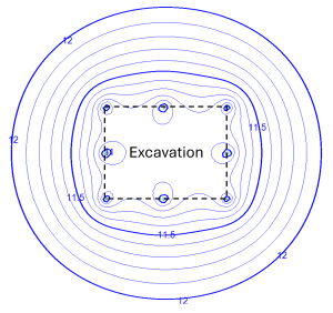
For the simulation, I used Anaqsim because of its flexibility and speed in setting up transient groundwater models. My model replicated the excavation as a large-diameter well equivalent to the pit area, with eight abstraction wells to simulate the dewatering system.
Here’s the process I followed:
- Initial Check: I first used constant-head wells to test if my configuration of eight wells could achieve the target drawdown. Both steady-state and transient simulations confirmed it could.
- Transient Simulation: Next, I simulated pumping at 689 m³/day (divided among the eight wells) over a 45-day period to compare results with the report’s predictions.
The Results
The simulation results revealed a significant discrepancy between the reported steady-state assumptions and the transient reality:
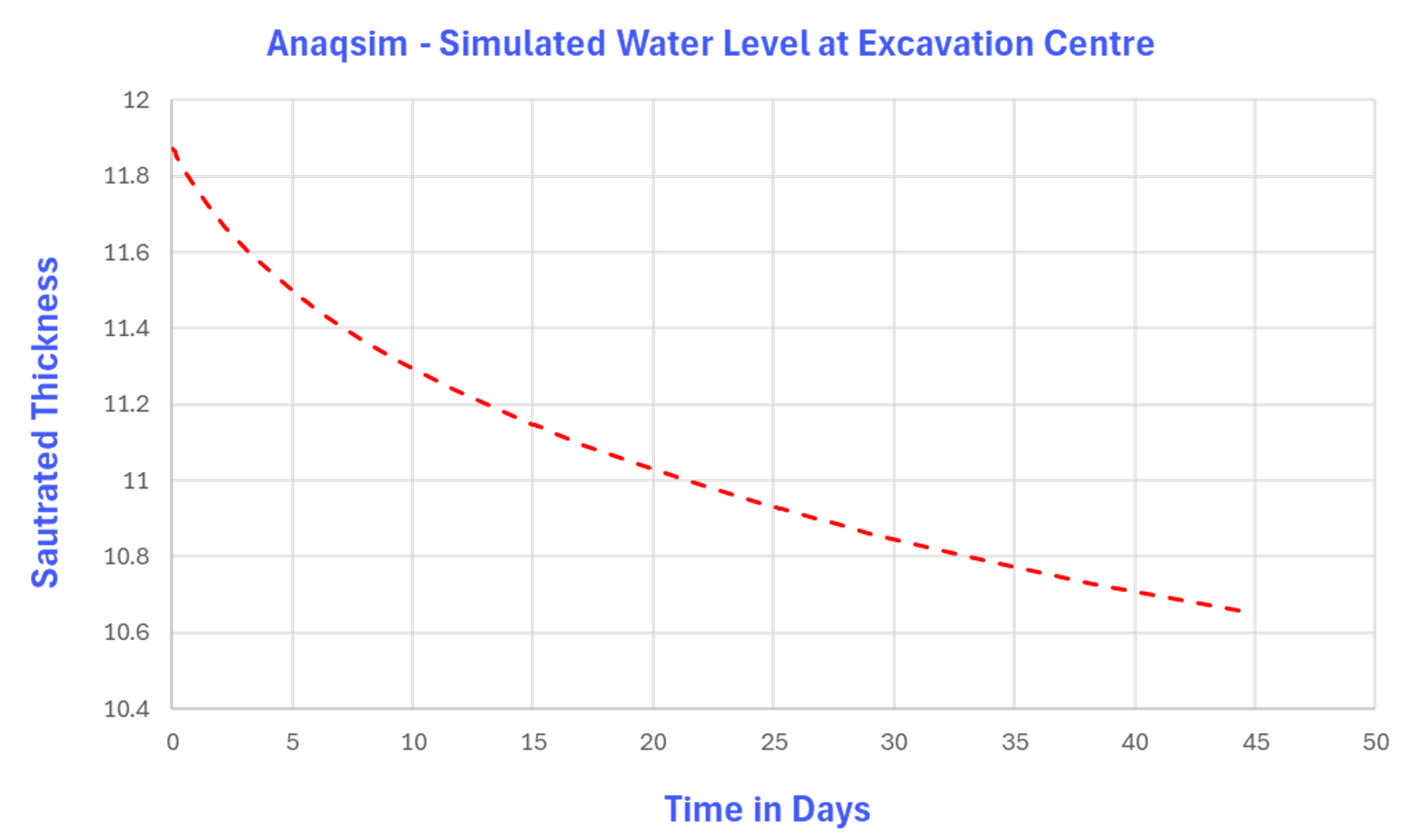
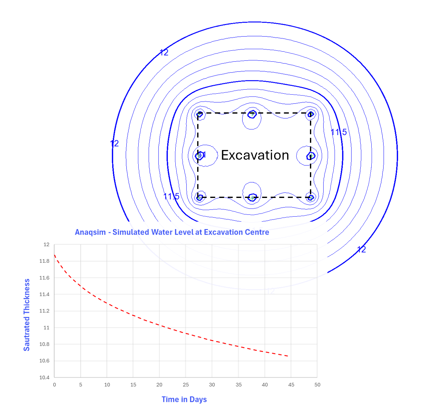
- Drawdown: After 45 days of pumping at 689 m³/day, water levels in and around the excavation remained at approximately 11.1 m—achieving less than 2 m of drawdown. This fell far short of the 3.5 m target.
- Observations: Using Anaqsim’s observation well feature, I tracked the drawdown at the center of the excavation. The results showed a gradual decline, indicating that reaching the target drawdown would take much longer than 45 days. I didn’t attempt to simulate it further but extrapolating from the time-drawdown curve it would take years to reach the target drawdown of 3.5 m at 689 m³/day.
Key Takeaways
This simulation highlights the risks of applying steady-state equations to short-term dewatering projects:
- Transient Conditions Matter: Dewatering typically begins in transient conditions. Steady-state assumptions can severely underestimate/overestimate the time required to achieve target drawdowns.
- The Role of Radius of Influence: The radius of influence is dynamic, not static, in transient scenarios. Relying on fixed boundaries can mislead the design process—a topic worth exploring in a future article.
Conclusion
The takeaway for engineers and practitioners is clear: To forecast and plan for immediate and short-term dewatering effects (i.e., days and weeks), transient simulations are essential. Calculations that rely on a constant radius of influence will either overestimate or underestimate actual dewatering rates, making project timelines and costs vulnerable to significant errors.